Gradient Descent and Backpropogation algorithm

SuperVised Learning

• Training a machine by showing examples instead of programming it explicitly.
• When the output is wrong, tweak the parameters of the machine.
• Works well for:
  • Speech → words
  • Image → categories
  • Potrait → name
  • Photo → caption
  • Text → topic
• Most of the practical applications of deep learning and AI in general use this paradigm.
• Eg: differentiation of images from car and airplanes.
• Works really well when we have lots of data to train our examples for.

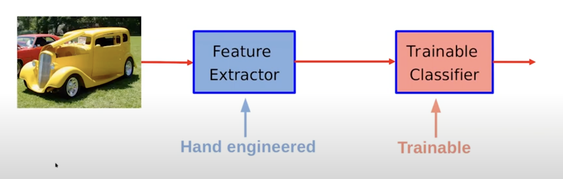
Standard Paradigm of Pattern Recognition and ML

• Born in the 1960s.
• part of the traditional Machine Learning
  • until the Deep Learning Revolution (2012)
  • 
  • The trainable classifier is where the learning takes part
  • Still popular , but superseeded by new algorithms using deep learning.

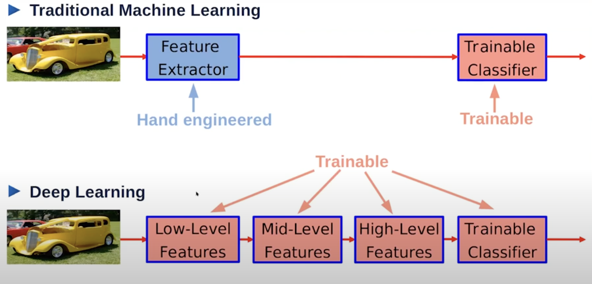
MultiLayer Neural Nets and Deep Learning

• Deep Learning has replaces the manual hand enigneered way of feature extractor using multi layers of neural networks which are trainable → hence called deep as the stack transforms the input into something else and then we train the entire system end to end.
• 
• The practical methods for this go back to a long time → the backpropogation algorithm.
• Took some time for this idea to percolate and for people to build machine learning system.

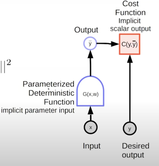
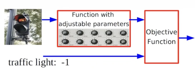
Parameterized Models:

• Parameterized Model → learning model, is basically a parameterized function.

$$\overline{y}=G(x,w)$$

• 
• This parameterized model produces a single output lets say a vector, matrix or tensor → generally something multidimensional or something like a sparse array representation or something like a graph.
• Both the input x, and output $\overline{y}$ are multidimensional arrays / tensors and these are parameterized by some parameters $w$ which are some knobs that we are going to adjust during training and these are basically going to determine the input/ output relationships bw input $x$ and predicted output $y$.
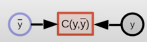
• Cost Function:
  • If any machine learning algorithm it will have an cost function.
  • The cost function in supervised learning as well as in other algorithms will compute the discrepencies, distance , divergence bw desired output $y$ and the $\overline{y}$ .
  • Eg: Linear Regression $$\overline{y}=\sum _i{w}_i{x}_{i}C(y,\overline{y})=||y-\overline{y}|{|}^2$$
    • here we are computing the square distance bw $y$ and $\overline{y}$.
    • This G may not be something simple to compute and something fixed number of steps and may involve minimizing the value wrt some other values.
  • Computing function G may involve complicated algorithms.

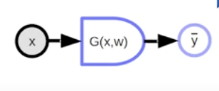
Block Diagram Notations for computation graphs

• Variables (tensor, scalar, continuous, discrete…)
  • observed: input, desired output…
    • 
  • computed variable: outputs of deterministic functions
    • 
• Deterministic Function:
  • 
  • Multiple Inputs and outputs (tensors,scalars,…)
  • Implicit parameter variable (here: w) that are tunable by training
• Scalar Valued Function(implicit output) → Cost Function :
  • 
  • Single Scalar Output (implicit)
  • used mostly for cost functions
• Symbolism kinda similar to graphical models → Factrographs
  • Graphical models dont care about the fact that you are directed models in one direction or the other.
  • Here we care about it.

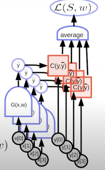
Loss Function, Average Loss:

• Machine learning consist in finding the $w$ that minizimizes the cost function averaged over the training set.
• A simple per-sample loss function:

$$L(x,y,w)=C(y,G(x,w))$$

• Training Set: Set of pairs, $x,y$ indexed by a index $P$ training samples and overall loss function that we have to minimize is equal to the discrepancy over the model $y$ and its output $\overline{y}$ .
• 
• A set of examples:

$$S=\{(x[p],y[p])/p=\mathrm{0....}P-1\}$$

• So the average loss over the set:

$$L(S,w)=1/P\sum _{(x,y)}L(x,y,w)=1/P\sum _{p=0}^{P-1}L(x[p],y[p],w)$$

• The avg operation computes the loss, we can write in terms of the graphs.

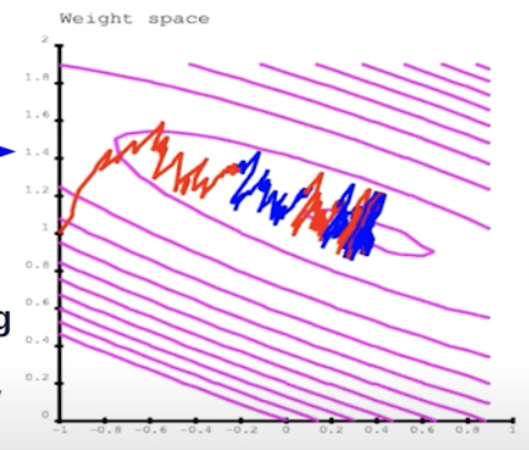
Supervised Machine Learning - Function Optimization

• Supervised machine learning and a lot of other machine learning can be just viewed as function optimizations.
• 
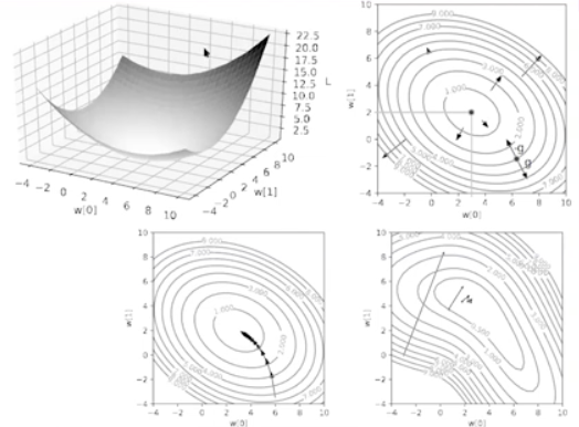
• It’s like walking in the mountains in a fog and following the direction of steepest descent to reach the village in the valley.
• But each sample gives us a noisy estimate of the direction. So our path is a bit random each time.
• 

$$W_i=W_i-\eta (\delta L(W,X)/(\delta W_i))$$

• Gradient based algorithms makes the assumptions that the functions are so much smooth and mostly differentiable - doesn’t have to be everywhere differentiable , have to be enough smooth so that local information about the slope should give the information where the minima is.
• The above image is method for Stochastic Gradient Descent. The process of SGD is:
  • Show an example
  • Run it through the machine
  • Compute the objective for that particular sample and then
  • Figure out how much and how to change the knobs to decrease the cost.

Gradient Descent:

• Full (batch) gradient: - This is actually very slow to compute. $$w=w-\eta (\delta L(S,w)/\delta w)$$
• Stochastic Gradient (SGD):
  • SGD exploits the redundancy in the samples:
    • Goes faster than full gradient in most cases for speed of convergence.
    • In practice, we use mini-batches for parallelization.
    • called stochastic as the evaluation of the single start point we get is a noisy estimate of the full gradient.
    • the avg of the full gradient is the averages of each of them.
    • Overall the avg trajectory would have the trajectory we would have followed by full gradient.
    • SGD exploits the redundancy bw the samples, and the faster you update the parameters the more easily you are able to exploit the redundancy bw these parameters. $$w=w-\eta (\delta L(x[p],y[p],w)/\delta w)$$
• 
• At the bottom the slope is zero and points towards the direction of the highest slope.
• These gradient based algorithms differ in:
  • How you compute the gradient ?
  • By what the $\eta$ size parameter is ?
    • Step-size parameter , that for simple things is decreased as we start reaching the minima.
    • For most of them, they are generally a Jaccobian positive definite matrix.
• In situations where the trajectory is more complicated, this could be entirely different in how we calculate the loss function.
• (TODO: 20:06)