RNN :
- Networks that was introduced before sequence to sequence jobs.
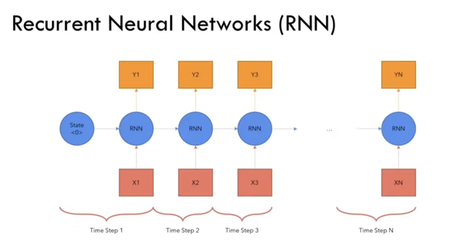
- They are allowed to map one sequence of input(X) to another sequence of output(Y). We split the sequence into different states X1,X2,… and pass onto the input RNN to generate Y1,Y2,.. and passed a initial state made up of 0s.
- The RNN → RNN connection is called the hidden state of the network , along with next input token and the network had to produce the next output token Y2, … and we extend it to Xn extending to Yn.
- If we have N tokens input, then we map for n tokens output.
- Problems with RNN:
- Slow computations for long sequences.
- Here we have do a for loop for the sequence , longer the sequence , longer the computation.
- Vanishing or exploding gradients:
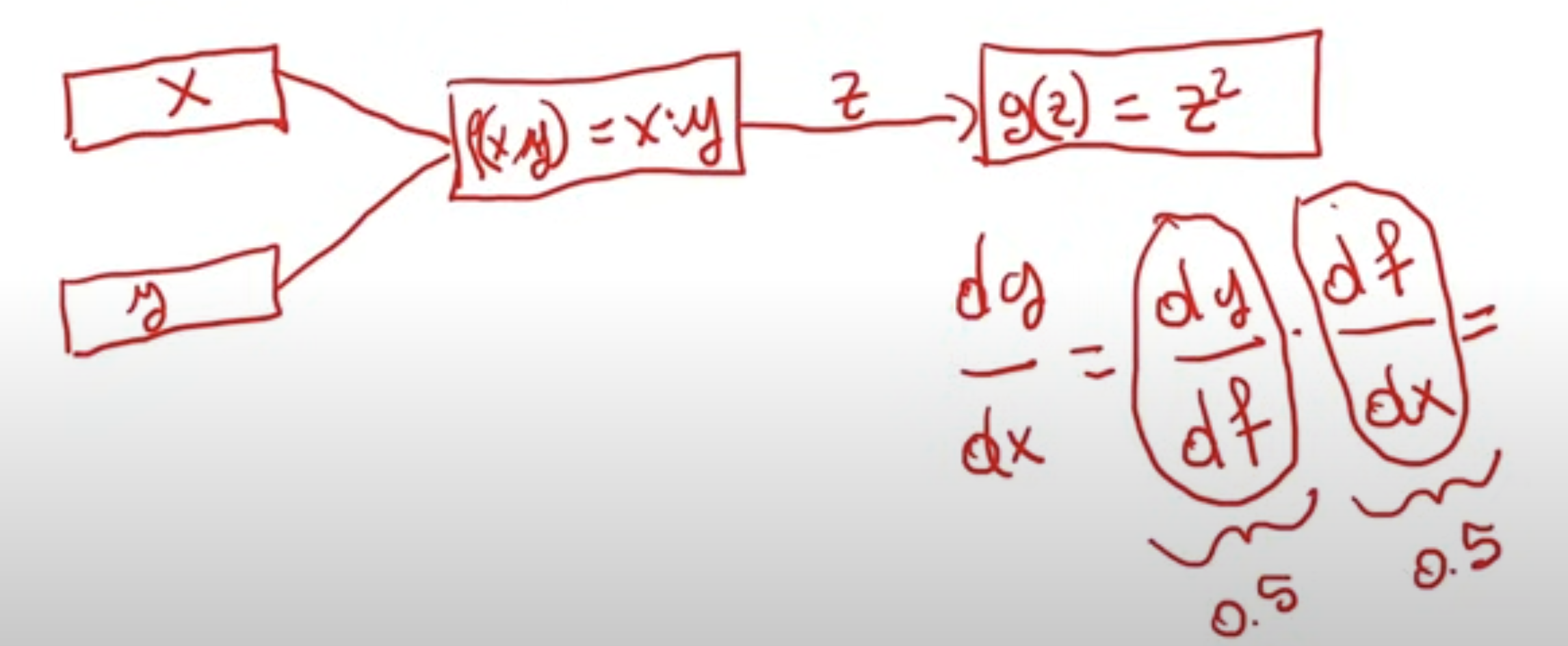
- PyTorch converts our network into computational graphs.
- PyTorch calculates the derivative of the loss function wrt to each weight.
- using chain rule we calcualte the derivative of each term, imagine if we have 1000 terms. Assume that the first term in this is 0.5 and the second term is also 0.5 , the resultant number will be a number that will be smaller than either of them( as each of them are smaller than 1). If we have a very big chain of computation, then it will either become a very big chain of number, or a very small number.
- and this is not desirable as our CPU/GPU can only repr our number till a certain bit → and our repr here wont be able to represent, and the weight will move very very slowly → gradient is vanishing.
- Difficulty in accessing information from long time ago (short context length)
- RNN is like a long graph of computation with a new hidden state.
- If we have a long computation, then the last token will have a hidden state whose contribution from the first token is nearly gone due to this long chain of multiplication. This will not depend much on the first token.
- Slow computations for long sequences.
Transformer :
- To address the issues of the RNN architecture, the transformer architecture was introduced.
transformer-architecture
⚠ Switch to EXCALIDRAW VIEW in the MORE OPTIONS menu of this document. ⚠ You can decompress Drawing data with the command palette: ‘Decompress current Excalidraw file’. For more info check in plugin settings under ‘Saving’
Excalidraw Data
Text Elements
Encoder
Decoder
Embedded Files
2fa089668e37f945f39d92a317f2cf10f27edf36: Screenshot 2024-12-28 at 10.42.40 PM.png
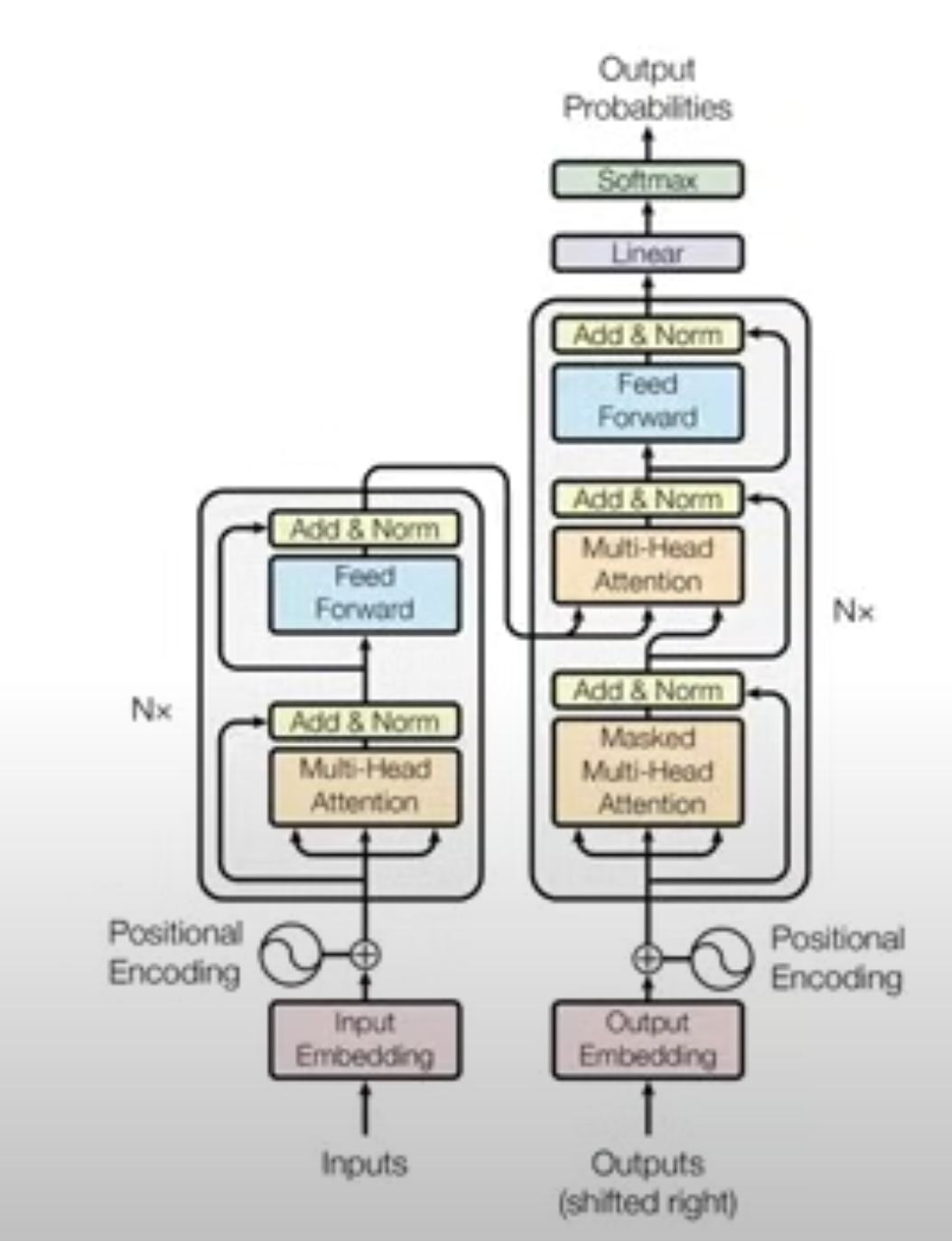
Link to original- The structure of the Transformer we can divide into 2 (major) parts:
- Encoder
- Decoder
- Linear Layer
- Encoder and Decoder are connected by a layer , where some output of the encoder is sent to the decoder.
- Encoder Layers:
- Starts with input embedding.
- Matrix Multiplication:
- Input Embedding:
- We transfer the input string into tokens → single words.
- not necessary into splitting into single words, we can even split the single tokens into multiple words.
- done in most transformer models.(by splitting each word into multiple words).
- for our example we are splitting a sentence into words.
- then map those words into a vocabulary (imagine we have a vocabulary of all the possible words that appear in our training set).This numbers are called as input ids.
- And map then to a vector of size 512 and always map the same word to the same mapping.
- Our input ids are parameters , the models will try to change these numbers according to the meaning of the word. Embedding will change according to the training process / loss function.
- 512 size → dModel
- Positional Encoding:
- We want each word to carry some information about its position in the sentence.
- we want the model to treat words that appear close to each other as “close” and words that are distant as “distant”.
- We want the positional encoding to represent a pattern that can be learned by the model.
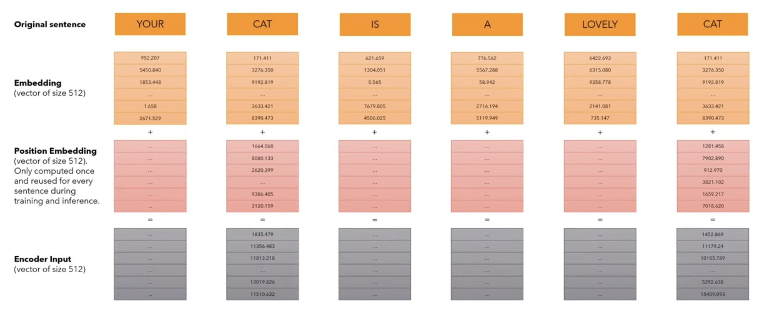
- we create positional encoding vectors that we add to these embeddings(size=512). 512 size (not learnt for the training process and is fixed.)→ gives an output of a vector of size 512. Computed once, and is fixed. This vector represents the position of the word inside of the sentence.
- How are these positional encoding calculated ?
- We create a vector of size 512 and for each position in this vector, we calculate the value using this 2 expressions:
- The first argument indicates the position of the word in the sentence.(here Your occupies 0).
- For the even dimensions we use the first formula, and for odd dimensions , we use the second formula, and we do this for all the words inside of the sentence.
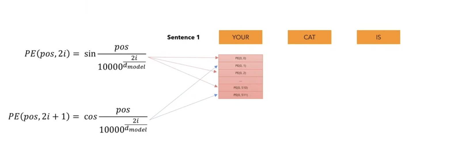
- If we have another sentence, we wont have another positional encoding and have the same, because the positional encoding are calculated once and used throughout both during inference and training.
- Why are we using trigonometric functions here ?
- Trigonometric functions like cos and sin naturally represent a pattern that the model can recognise as continuous, so relative positions are easier to see for the model. By watching the plot of these functions, we can also see a regular pattern. so we can hypothesise that the model will see it too.
- Multi-head Attention:
- For the purpose of understanding now, we are going to use a single head self-attention and then progress towards multi-head attention.
- What is Self-Attention ?
- Mechanism that existed before.
- Self attention allows the model to relate words to each other.
- Input embeddings that captured the meaning of the word.
- Positional encoding that give the information about the position of the word in the sentence.
- Now we want the self attention to relate words to each other.
- Consider a simple case , where we consider the sequence length seq = 6 and and the matrices Q,K,V are just the input sentences.(K is just the transpose of Q)
- We calculate the self attention from the formula above to calculate the relation of the word to others in the same sentence.
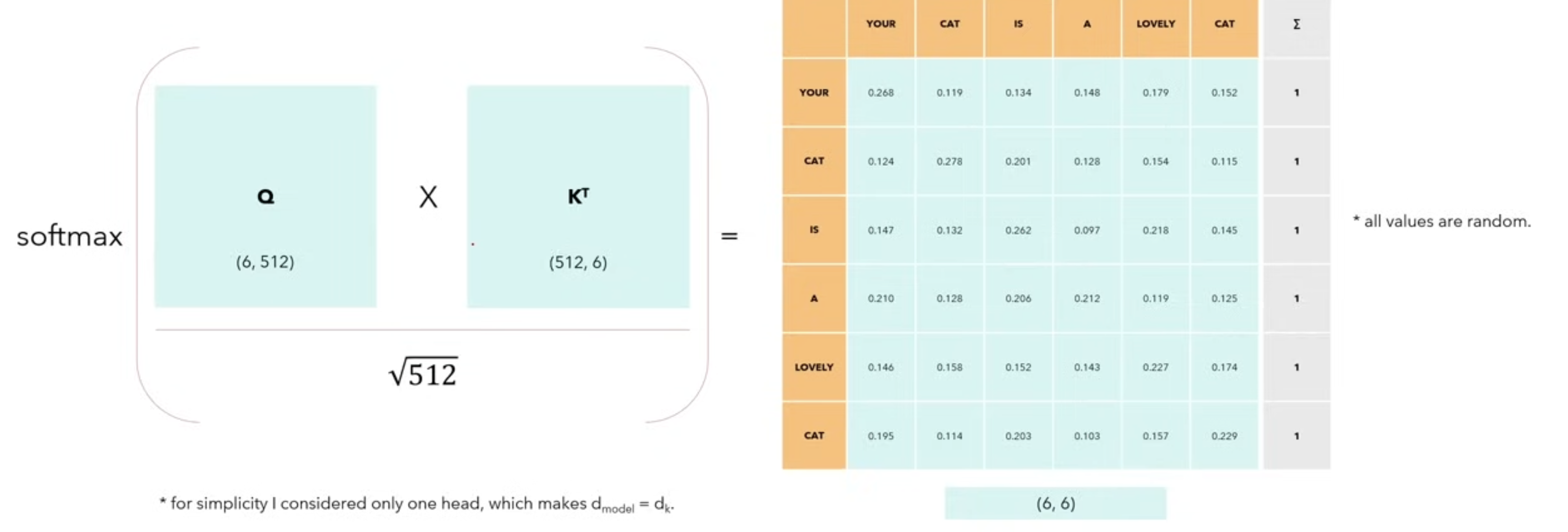
- Each value in the matrix of the first row with first col, first row with first col etc. The softmax makes all the values in such a way that they sum upto 1.
- Multiplying By V:
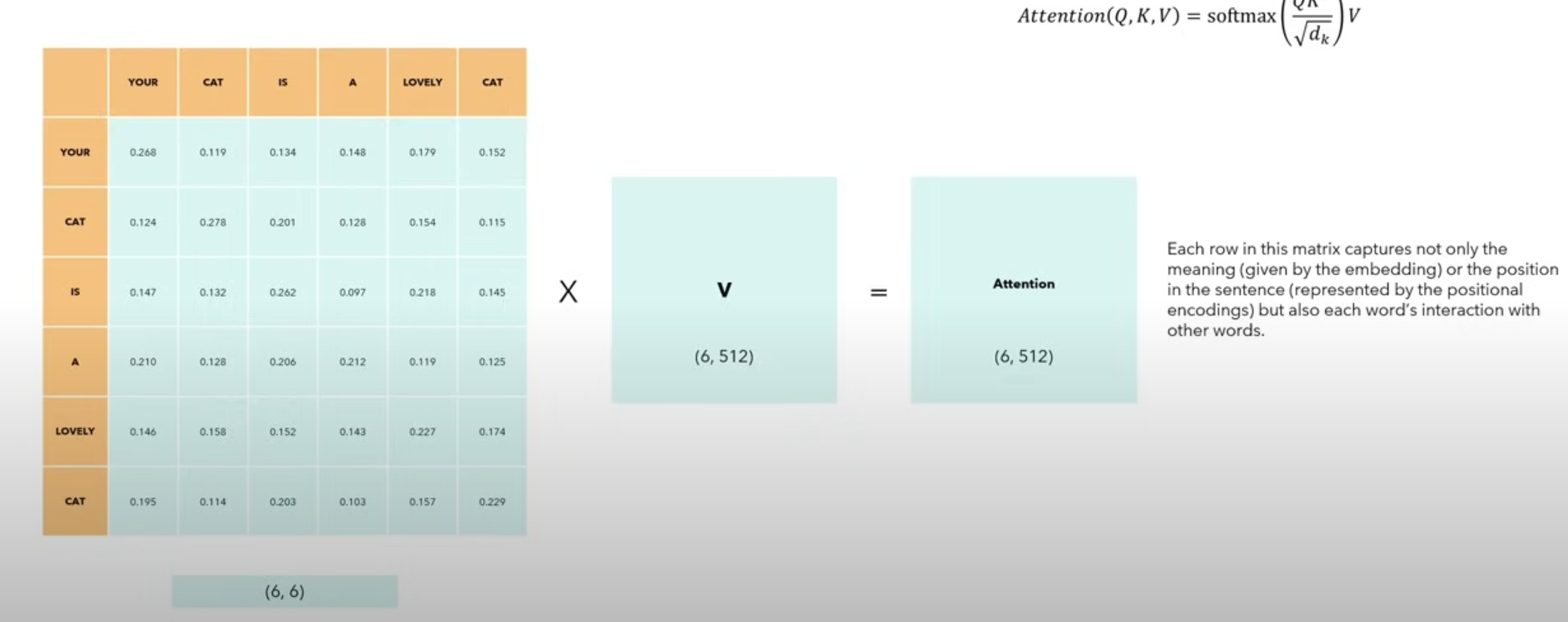
- The dimension of the Attention matrix is the same as the dimension of the matrix that we started from. This means that we obtain new matrix of 6 rows and 512 cols and so we have 6 words and each words having a embedding of dimension 512, so now this embedding represents not only the meaning of the word, not only the position , but rather it is a special embedding that captures the relationship of the word in relation to all the other words.
- Self attention properties:
- Self attention is permutation invariant.
- if means that if for a matrix A and its corresponding result matrix A’ , if we change the rows of a matrix, the same rows of matrix A’ will change accordingly. But the values in each property will not change values.
- Self attention does not require any parameters. Until now the interaction between words has been driven by their embeddings and the positional encodings. This will change later.
- we expect values along the diagonal to be the highest.
- as it is the dot product of each value with itself.
- If we don’t want some positions to interact , we can always set their values to before applying the softmax in this matrix and the model will not learn those interactions. We will use this in the decoder.
- Self attention is permutation invariant.
- Multi-head Attention:
- Imagine we have our encoder and our input sentence (6*512) dmodel is the size of the embedding vector, we make 4 copies of it and h = number of heads,
- (continue from 29:35)https://www.youtube.com/watch?v=bCz4OMemCcA